Plotting: showing, saving, manipulating, adding styles

Showing, saving, and manpipulating plots is easy. All thebeat’s plotting functions internally use matplotlib.

Showing a plot

How to show a plot depends on whether you are using Python in an interactive environment or as a stand-alone script. If you run Python code line by line, it is likely that you’re in interactive mode. If you run an entire Python script at once (e.g. by running python script.py in a terminal), you will be in non-interactive mode.

Examples of interactive environments are, e.g., Jupyter notebooks or the interactive mode of Spyder.

Interactive mode (e.g. Jupyter notebooks)

In interactive mode, plots will be displayed automatically when calling any of thebeat’s plotting functions:

import thebeat
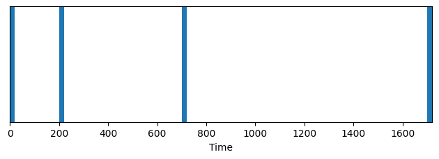
seq = thebeat.Sequence([200, 500, 1000])
seq.plot_sequence()

(<Figure size 640x240 with 1 Axes>, <Axes: xlabel='Time'>)

Together with the plot, we see the so-called repr of the plot printed. If you want to suppress this, in Jupyter notebooks you can add a semicolon at the end of the function, i.e. seq.plot_sequence();.

Non-interactive mode

When you’re running code as a separate script (i.e. in non-interactive mode) in order for the plot to show, we must first import matplotlib.pyplot and run its .show() method after creating the plot, as follows:

import thebeat
import matplotlib.pyplot as plt

seq = thebeat.Sequence([200, 500, 1000])
seq.plot_sequence()  # The plot is created, but not shown
plt.show()  # Show the plot

---

Adding a style/theme to the plot

For adding an existing style to a plot we can do one of two things:

1. We use a ‘context manager’ to temporarily set the style, make the plot we want, and then continue in the default style.

2. Set the theme options globally in the document. Note that until Matplotlib is imported again, this style will apply to all plots (created by thebeat, Matplotlib, or something else that uses Matplotlib internally).

There’s standard Matplotlib styles that we can use, or we can use the (slightly prettier) standard styles from Seaborn. Both options are illustrated below, note that you have to install Seaborn separately in order to use those styles (using e.g. pip install seaborn).

Temporarily use a different style

# Using a Matplotlib style
import thebeat
import matplotlib.pyplot as plt

seq = thebeat.Sequence(iois=[200, 500, 1000])

# Plot using a context manager
with plt.style.context('ggplot'):
    seq.plot_sequence()

# Using a Seaborn style
import thebeat
import seaborn as sns

seq = thebeat.Sequence(iois=[200, 500, 1000])

# Plot using Seaborn's context manager
with sns.axes_style('dark'):
    seq.plot_sequence()

Set style globally

# Using a Matplotlib style globally
import thebeat
import matplotlib.pyplot as plt

plt.style.use('ggplot')

# Using a Seaborn style globally
import thebeat
import seaborn as sns

sns.set_style('dark')

---

Saving plots

All thebeat’s plotting functions return a :class:matplotlib.figure.Figure object, representing the entire plot, and a :class:matplotlib.axes.Axes object, which represents the actual graph in the plot. These objects we can use to show, save or manipulate the plots.

In the example below we create a recurrence plot, and save it to disk using savefig(). We ask for a plot with a dpi of 600, so we get better quality.

from thebeat import Sequence
from thebeat.visualization import recurrence_plot

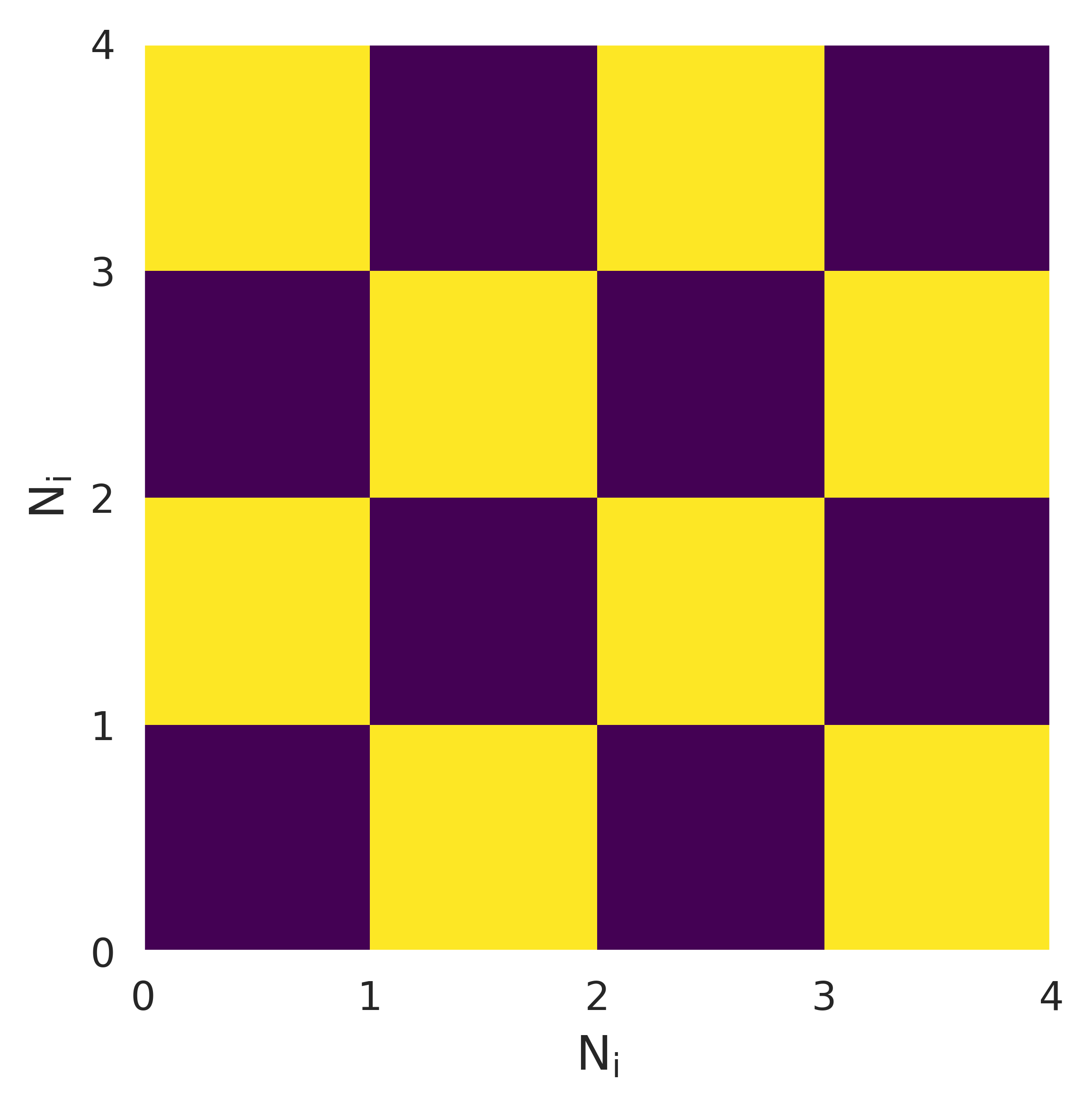
seq = Sequence(iois=[300, 400, 300, 400])
fig, ax = recurrence_plot(seq, dpi=600)
fig.savefig('recurrence_plot.png')

Adding in title, x_axis label etc.

thebeat’s plotting functions contain a few arguments for commonly encountered manipulations, such as adding in a title, changing the figure size, etc. These are the so-called keyword arguments (**kwargs).

To see a list of available keyword arguments, see e.g. thebeat.helpers.plot_single_sequence().

Manipulating plots

Manipulating plots works similarly. We can use the resulting matplotlib.figure.Figure and matplotlib.axes.Axes objects for manipulation, and only show the figure afterwards.

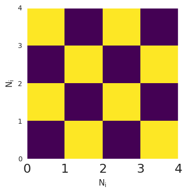
fig, ax = recurrence_plot(seq)
ax.set_xticklabels([0, 1, 2, 3, 4], fontsize=18)
fig.show()

/tmp/ipykernel_2297/841921616.py:2: UserWarning: set_ticklabels() should only be used with a fixed number of ticks, i.e. after set_ticks() or using a FixedLocator.
  ax.set_xticklabels([0, 1, 2, 3, 4], fontsize=18)

More info on how to manipulate plots can be found in the matplotlib documentation.